Forecasting at Scale
Prologue
Time-series forecasting is a widely adopted practice in many businesses that produce and store temporal measurements. Often, the scale of the business problem causes a variety of problems in producing reliable and interpretable forecasts. Such problems include the volume, variety and quality of time-series data which makes it challenging to train intrepretable predictive models.
A similar challenge is faced during the production of cinematic music due to the variation in the number and duration of scenes. Composers use a clever technique to tackle this problem, which can be replicated by Data Scientists to build a robust forecasting framework at scale. To understand how, continue reading by acknowledging that you are familiar with fundamentals of time-series. If you need a refresher, go through my time-series primer.
 Photo by Vienna Reyes on Unsplash
The Scale
Tackling the sheer volume of time-series variables and the associated variety and data quality issues remain as the significant challenge in forecasting problems. The number of time-series variables can range from tens of tens to tens of thousands to tens of millions. This post addresses the scale of devising an appropriate framework to train and interpret models for each variable when there are several variables. The scale of engineering a distributed computing system for fast and efficient model training shall be addressed in a different post in future.
The brute force approach is to use an AutoMLesque time-series forecasting package for all variables, given one has the luxury of hardware. Such a package would select the best performing model for each variable and doing so would have solved only half the problem. Often, accuracy alone is not sufficient to justify interpretability of models. A robust forecasting framework has to embody accuracy as well as interpretability. To build one, data scientists can replicate the cinematic music production technique.
The technique
In cinematic music production, a theme song is composed to be the signature music associated to the overall story. Specific tracks are composed for prominent locations or characters in the story. For each scene, the music will be a mix of theme song and character/ location tracks. The duration of score will not scale proportionally with the duration of movie. To replicate this technique, Data Scientists need to identify the theme of the forecasting problem at hand and map time-series variables into few relatable characters.
The theme of the forecasting problem can be defined by answering the following questions:
- Meaningful history
- Zeroes vs Missing values
- Suitable validation rule book
Select a tab to view relevant information
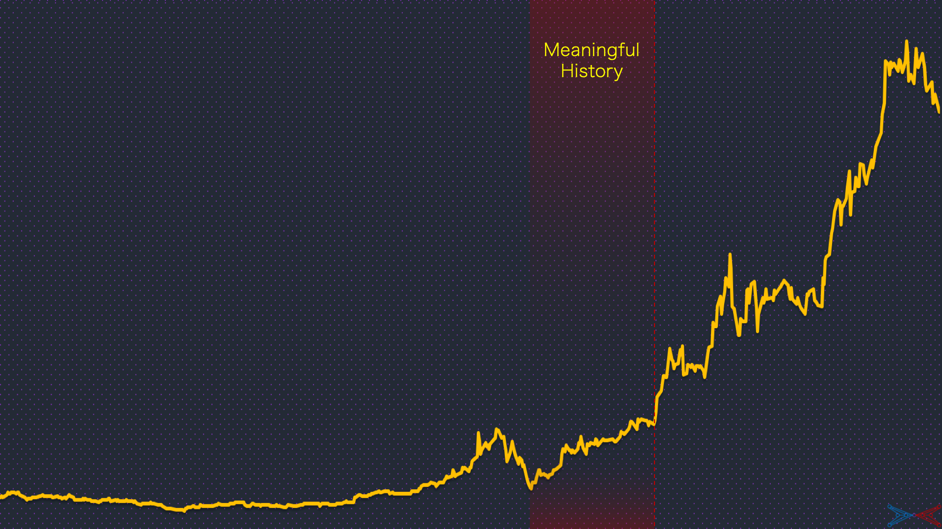
Meaningful history is the amount of historical data suitable and useful for training. This parameter can be determined using grid search which will be computationally expensive at scale. However, given the dynamic nature of most businesses, there can be multiple changepoints in the time-series. The frequency of changepoints needs to be assessed for determining an appropriate start. If there are multiple valid starts to choose from, then grid search can be applied to select one.
A classic example is a stock-price prediction problem with years of data available but not useful in entirety for predicting future prices. In another situation with an objective of predicting user footprint volume, the definition of user footprints could change with time, implying not all historical observations are useful for training.
These are the problems faced when data is abundant. If it is not, the models will be subject to high bias or variance. To prove or disprove that, business-driven definition of meaningful history can be helpful. Also, it is a good practice to include a few rule-based and naive algorithms in the AutoML package to deal with varying data sizes.
The rationale behind the presence of missing values needs to be investigated to decide on the right treatment procedure. It is further more important to differentiate zeroes from missing values in the context of business.
In weather forecasting, a value of zero is possible and different from missing values. The missing values would have appeared due to equipment failure or data loss among a multitude of reasons. In such cases, they have to be treated differently from zeroes. Consider a demand forecasting problem where zero demand indicates no demand. Here, zeroes may have the same meaning as the missing values do and they can be treated similarly.
Missing values represent the intermittency of time-series and their treatment will alter its distribution. The models aren't trained with right data if zeroes and missing values are treated inappropriately.

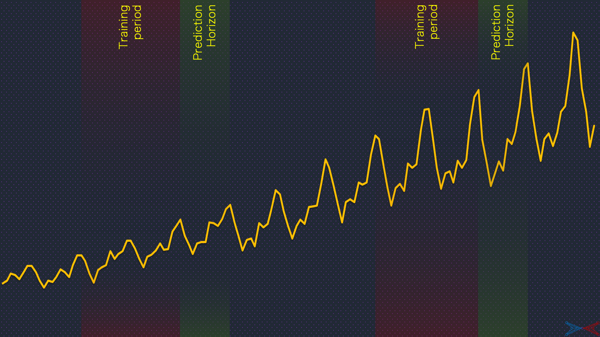
A right validation procedure for a forecasting framework quantifies its potential to solve the business problem. The validation can be done right by approximating the business problem as a real-valued function of time-series variables. The uncertainity associated with the values of this function is derivable from the individual model errors.
For time-series variables, there are several metrics to evaluate accuracy. Sometimes, MAPE is more suitable if the error needs to be quantified on a relative scale. However, MABS can be more meaningful in situations where MAPE will be consistently larger due to the scale of values. A combination of traditional accuracy metrics shall be robust enough for any variable irrespective of its distribution. The uncertainity associated with the function of time-series variables can be estimated by applying the theory of random variables or simpler heuristics.
Consider a hierarchical forecasting problem where the volume of units sold is forecasted with an objective of estimating cumulative revenue. The errors made by the individual models can be small, but the error made on revenue estimation by adding the individual predictions is unknown. Also, scale of unit-volumes might significantly differ from the scale of revenues. Traditional accuracy metrics like MAPE might get enlarged or shrunk in translation if the relationship between unit-volume and revenue is not linear. Unless computed, the performance of individual models cannot be correlated with the performance of forecasting system.
Moreover, the validation procedure is not straight-forward in time-series forecasting, with the notion of k-fold cross validation being invalid. There will be a few data transformation steps to be done before training and validation, depending on the model. A detailed post on the model validation in time-series forecasting shall be published soon.
The answers to these three questions signify the action plan for treatment of historical data and validation of forecast accuracy. This is the act of composing the theme song. The next step is the composition of character specific tunes.
Time-series classification
Before unleashing the AutoML, the time-series variables can be classified into a few characters based on their properties. Time-series clustering is a paradigm with ample scope for application of sophisticated algorithms. But the grounded approach presented in Syntetos et al (2005) is practical in a lot of situations, runs in a flash and comprehensible for business leaders. Let’s fire up the hardware during model training, shall we?
Syntetos et al (2005) classifies the time-series variables based on their intermittency and variance. The metrics to quantify intermittency and variance are:
-
Average demand interval (ADI) -
Coefficient of Variation squared (CV2)
Average demand interval is the ratio of total number of timestamps in the observation period to the number of timestamps with non-null values. Coefficient of Variation (squared) is the squared ratio of standard deviation to the mean of observations that are not nulls.
Null values are present in time-series when no real-value has been observed at certain timestamps. The presence of missing values due to data loss or observational failure is a different situation that has to be dealt through imputation.
The time-series variables shall be classified as illustrated below:
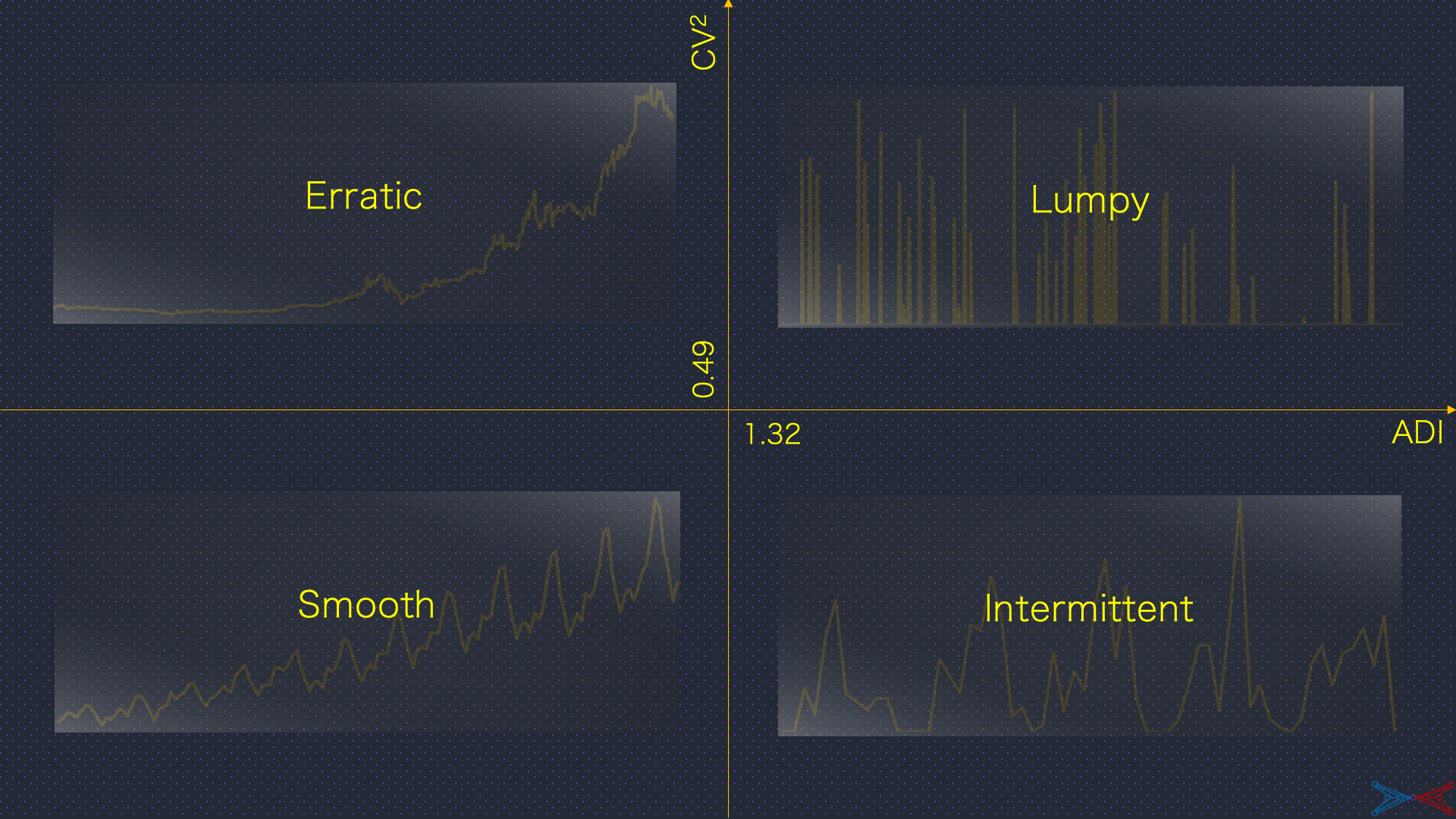
The boundary conditions on ADI and CV2 are mathematically dervied and stastically tested with 3000 time-series. They can be modified to have fewer time-series classified smooth or intermittent. The following tabs describe the practicality of this classification:
A time-series is smooth if its ADI <= 1.32 and CV2 <= 0.49. The conditions imply the small variance and presence of nearly no null values in the time-series. Traditional forecasting models can achieve high prediction accuracy over smooth time-series. The plot below shows a time-series which is smooth:
The AutoML can be configured to have predominatly more traditional algorithms for smooth time-series. As a step further, smooth can classified into "very smooth", "quite smooth" and "barely smooth" sub-classes based on CV2. This sub-classification enhances the model selection further as superior forecasting models with capability to learn strong seasonal effects are only ever required for the last two sub-classes.
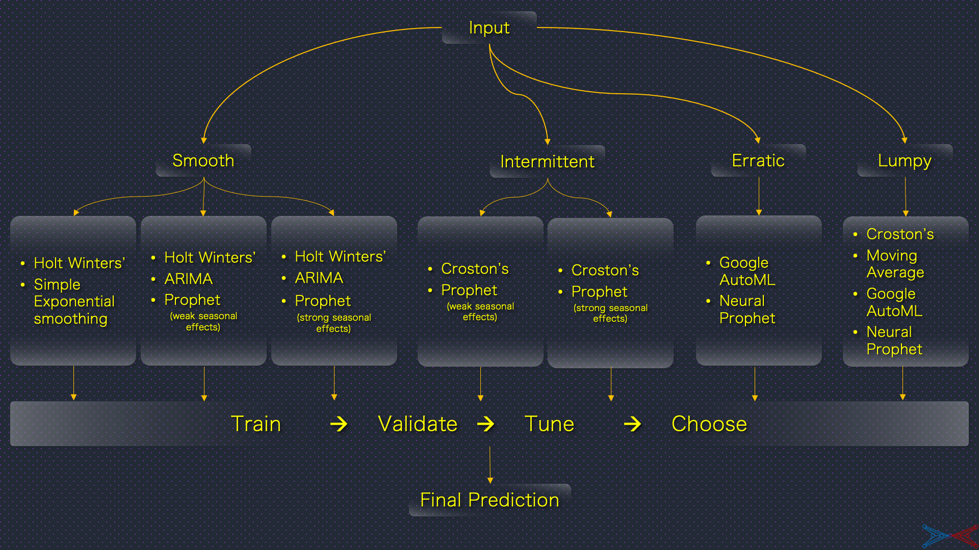
Facebook's Prophet with its seasonality and holiday components is a flexible formulation to tackle a range of predictable seasonal/ cyclic effects. A combination of STL decomposition, Auto-ARIMA and variants of Prophet (mild, moderate and strong seasonal effects) shall be robust enough to tame the variances in smooth time-series.
A time-series is intermittent if the ADI > 1.32 and CV2 <= 0.49. The conditions imply the small variance but presence of significant number of null values in the time-series. Traditional forecasting models capable of dealing intermittency can achieve reasonable prediction accuracy. The plot below shows a time-series which is intermittent:
Even for intermittent time-series, the AutoML can be configured to have more traditional algorithms than sophisticated ones. The sub-classification into "very intermittent", "quite intermittent" and "barely intermittent" shall be based on ADI. Superior traditional algorithms are required only for the first two sub-classes. A combination of Croston's model and variants of Prophet shall be sufficient for intermittent time-series.
A time-series is erratic if its ADI <= 1.32 and CV2 > 0.49. The conditions imply the high variance and presence of nearly no null values in the time-series. The high variance could not be explainable by time dimension alone and hence it is generally not possible to achieve a reasonable prediction accuracy with traditional forecasting models. The plot below shows a time-series which is erratic:
For erratic time-series, advanced time-series clustering algorithms are required for further sub-classification. The AutoML package can be configured to activate several neurons. This is the paradigm to unleash the RNNs, autoencoders and the likes. Moreover, the varinace may not be largely explainable by time and usage of external regressors can improve accuracy further. The next section briefly explains the addition of external regressors to forecasting models.
Google debuted a time-series AutoML package in 2020 backed with a tall claim that it outperforms 92% of hand-crafted models for several kaggle datasets. Facebook debuted NeuralProphet, the gen-next update to the proven Prophet model. Given the availability of hardware, a combination of Google AutoML and NeuralProphet shall be a force to reckon with for erratic time-series.
Although, Google and Facbook termed the compute costs to be moderate, such claims will always remain subjective. But selective application of AutoML and NeuralProphet for erratic time-series will reduce the hardware requirement further.
A time-series is lumpy if its ADI > 1.32 and CV2 > 0.49. The conditions imply the high variance but presence of significant number of null values in the time-series. There is too much variation and too little data to achieve a reasonable prediction accuracy. The plot below shows a time-series which is lumpy:
For lumpy time-series, it's either the rule-based/naive or the black-box algorithms that can learn some pattern from the sparse observations. A combination of Croston's model, Google AutoML and NeuralProphet shall be robust enough for this class.
All in all, time-series classification is a divide and conquer design pattern for forecasting at scale. It not only optimizes runtime & memory but also enhances the overall interpretability of the forecasting framework. The classification of time-series variables is the act of associating them with 4-10 characters. Configuration of AutoML for each sub-class is the act of composing tunes for each character.
The Framework
The illustration below summarises the framework for mixing the theme song and the character tracks. This forecasting framework is scalable along its length and breadth. It is applicable for any number of time-series variables and its robustness shall be further enhanced with selective addition of more suitable algorithms without raising the compute costs on a disproportionate scale.
Epilogue
This is the framework my use case deserves,
but not the one it needs right now.
So, I have pinned it to a blog post,
so that someone will use it
because it’s not just a framework,
it’s a silent predictor, a watchful detector,
A Dark Knight!